Colligative properties of solutions

What are the colligative properties of solutions?

When a solute is dissolved in a solvent, some properties of this solvent are modified, such as vapor pressure, boiling point, melting point and osmotic pressure.

These properties are known as colligative properties. The extent to which these modifications occur will depend on both the concentration and the nature of the solute. Some examples of common colligative properties are described below, depending on the type of solute present.

Solutions with volatile components

Vapor pressure

Let us imagine that we have a liquid in a container. The molecules on the surface can leave the liquid phase and move to the vapor phase, placing themselves on top of the liquids and exerting a pressure on them called vapor pressure.

As the gas-phase molecules increase, the vapor pressure of the liquid will increase.  There will come a time when the vapor pressure equals the atmospheric pressure.

P_vap = P_at

A phase change will appear as the boiling point of the liquid will have been reached.

If instead of having a single liquid in the vessel we have a binary solution, two things can happen, that it behaves as an ideal solution or as non-ideal, i.e., interactions occur between the two liquids.

Ideal binary solution

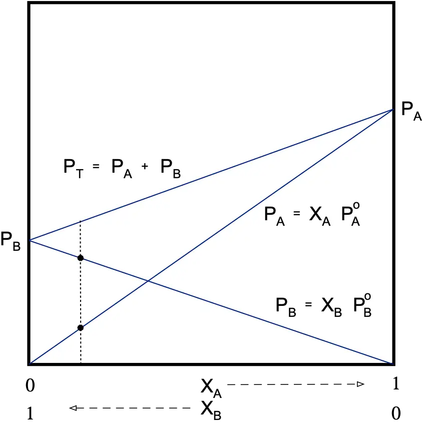
The components will be equally distributed throughout the mass of the solution, there being neither attractive nor repulsive interactions between them, so that the tendency to pass to the vapor phase will be the same in both.  The total vapor pressure will be equal to the sum of the partial vapor pressures of the components:

P_T =P_A + P_B

Experimentally, it is shown that an ideal solution satisfies Raoult’s law:

P_A =X_A·Pº_A

Pº_A = vapor pressure of the pure component

X_A = mole fraction

Therefore:

P_T =P_A + P_B = X_A·Pº_A + X_B·Pº_B

It is true that the pressure of a component in solution is lower than when this component is pure.

P_A < Pº_A          and          P_B < Pº_B

This indicates that P_T of the solution will always be between the vapor pressures of the components that form it.

From the component pressures the mole fractions of the components can be calculated:

P_T =P_A + P_B = X_A·Pº_A + X_B·Pº_B

X_A = 1 – X_B

X_B = 1 – X_A

P_T =P_A + P_B = X_A·Pº_A + (1-X_A)·Pº_B

P_T = X_A·Pº_A + Pº_B – X_A·Pº_B = X_A·(Pº_A – Pº_B) + Pº_B

X_A = (P_T-Pº_B)/ (Pº_A – Pº_B)

X_B = (P_T-Pº_A)/ (Pº_B – Pº_A)

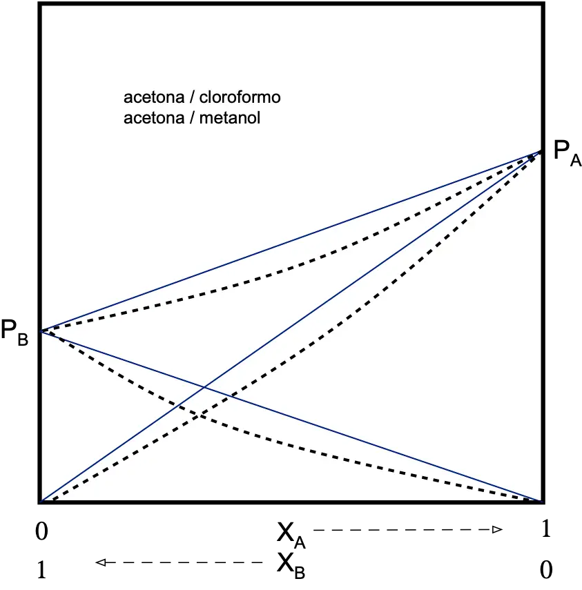
Non-ideal binary dissolution

There can be two types of interactions, attractive or repulsive.

Attractive (negative deviation)

The tendency to escape to the gas phase will be less than that of an ideal solution.

P_A < X_A·Pº_A

P_B < X_B·Pº_B

Therefore, the total vapor pressure of the solution will be lower than that predicted by Raoult’s law.

P_T < P_Raoult

The deviation from Raoult’s law is measured by a coefficient called “activity” (γ). The activity (γ) is equal to the actual pressure of a component divided by its theoretical Raoult’s law pressure.

γ_A=P_A/X_A·Pº_A                         γ_A ≤ 1   γ_B ≤ 1

Real solutions only behave ideally when they are very dilute.  Real gases have ideal behavior at low pressures and high temperatures.

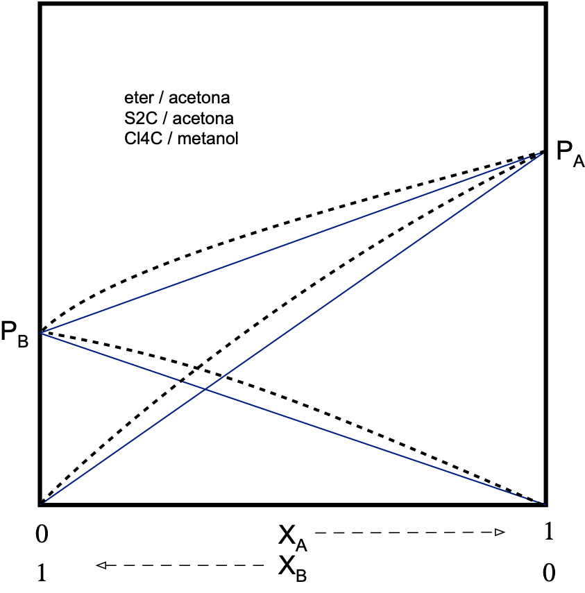
Repulsive (positive deviation)

There will be a repulsion between the components of the solution so that the tendency to escape to the vapor phase will be greater than in the case of an ideal solution.

The P of the dissolution will be higher than that provided for in the Raoult’s law.

P_A > X_A·Pº_A

P_B > X_B·Pº_B

P_T > P_Raoult                  and          γ_A ≥ 1 γ_B ≥ 1

Boiling point

Temperature at which the vapor pressure (of a solution in this case) becomes equal to the external pressure.

Ideal binary solution

• When the partial pressure of component B is greater than that of A: Pº_B > Pº_A. Component A will be the least volatile and will be less present in the gas phase.

• Otherwise: Pº_A > Pº_B

Component A will be the most volatile and will be more present in the gas phase.

So if we increase the pressure, the vapor will be enriched in the more volatile component and the solution in the less volatile component, so we can separate both components.

In practice this would be a difficult procedure to separate both components, so it is easier to increase the temperature, since the component that has a higher vapor pressure has a lower boiling temperature.  This procedure is called distillation.

Non-ideal binary dissolution

Solutions with attractive or repulsive interactions cannot be completely separated by the distillation procedure.

Only one of the components can be separated pure, the other being mixed with a defined composition called azeotrope.

In solutions with attractive interactions the azeotrope has the maximum boiling temperature higher than that of the pure components.  In solutions with repulsive interactions the azeotrope has the highest boiling temperature higher than that of the pure components.

Mixtures of immiscible components

Since there is no dissolution between the two solvents, each component will retain its properties, so the vapor pressure will be the sum of the vapor pressures of each of the pure components.

P_T = P_A + P_B = Pº_A + Pº_B

P_T will be greater than each of the partial pressures of the components of the mixture:

P_T > Pº_A                      P_T > Pº_B

And therefore, the boiling temperature of the mixture will be lower than the boiling temperatures of each of the pure components.

Example: Mixture of water and oil.

T_e H₂O = 100 ºC

T_e oil = 350 ºC

T_e total < 100 ºC

The vapor pressure of the mixture and therefore its boiling temperature will be constant, since they do not depend on the mole fractions of the components.

The fact that the mixture always boils at a lower temperature can be used for the distillation of components with high boiling points.

When water is used the technique is called “steam distillation”.

We can see the quantitative relationship between the pressures of each of the components as follows.

According to Dalton’s Law:

P_i = Y_i·P

for two components the relationship would be:

(Pº_to / Pº_to) = (Y_to·P_t) / (Y_b·P_t) ⇒

Pº_to / Pº_b = Y_b / Y_b  = (n_to/n_t) /(n_b/n_t) = n_to / n_b  = (m_to/M_to) / (m_b/M_b)   ⇒

M_a being the molar mass of compound a and M_b the molar mass of compound b.

Pº_to / Pº_b = (m_to· M_b) / (m_b ·M_to) ⇒

M_a =(m_a· Pº_b · M_b) / (m_b · Pº_a)

It is not common to measure “molar mass” from partial pressures, because it is very expensive.

For example: nitrobenzene has a boiling point 218.8 and density 1.0203 g/cm³. Water has a boiling point of 100 ºC and density 1.0 g/cm³.

However, another more useful expression can be extracted from the above equation. Thus, it allows us to relate the distilled masses and they are directly proportional to the vapor pressures and molar mass of each of the components.

(m_a/m_b) = (Pº_a / Pº_b) · (M_a / M_b)

Solutions with non-volatile solute

The total vapor pressure will be due only to the partial vapor pressure of the solvent.

P_T = P_D + P_S = X_D Pº_D + X_S Pº_S                           (Pº_S = 0)

P_T = X_D Pº_D

We will see the colligative properties of these solutions under ideal conditions, i.e. when they are diluted.

Vapor pressure

P_T = X_D Pº_D

Since the mole fraction of the solvent will vary between 0 and 1, we will have Pº_D > P_T

Therefore, the effect of the addition of a non-volatile solute is to reduce the vapor pressure of the solvent.

The molecular weight of a non-volatile solute can be determined from the vapor pressure of the solution from that of the pure solvent:

P_T = X_D Pº_D = (1 – X_S) Pº_D = Pº_D – X_S Pº_D

X_S = (Pº_D – P_T)/Pº_D = n_s/n_t ≈ n_s/n_d                    (n_s << n_d in diluted solutions)

pm_S = [Pº_D/(Pº_D – P_T)] m_S·pm_D/ m_D

pm_S = [Pº_D/(Pº_D – P_T)] m_S·pm_D/ m_D

Boiling point

The boiling point is the temperature at which the vapor pressure is equal to the external atmospheric pressure.  Adding a non-volatile solute to a solution increases the boiling temperature of the solution. A rise in the boiling point of the solvent occurs.

This increase in boiling temperature (ΔT_e) is defined as the difference between the boiling point of the solution (T_es) and the boiling point of the pure solvent (T_ed):

ΔT_e = T_es – T_ed

This increase in temperature will be related to the decrease in vapor pressure of a solvent when a non-volatile solute is added to it.

ΔP = Pº_D – P_T

so that:

(Pº_D – P_T)/ ΔT_e = K                             ΔT_e = (Pº_D – P_T)/K

the rise in boiling point will be proportional to the amount of solute added, i.e. the mole fraction of solute:

ΔT_e = X_S·(Pº_D/K) = X_S · K’                                X_S = (Pº_D – P_T)/Pº_D

The increase in boiling point can also be related to the molality:

X_S = n_s/n_t » n_s/n_d = n_s·pm_D/m_D                       (n_s<<n_d in diluted solutions)

m = n_s/(m_D/1000) = 1000n_s/m_D

X_S = m·pm_D/1000

In this way

ΔT_e = K’·X_S = m·(pm_D·K’/1000) = m K_e (K_e = molal ebulloscopic cte)

K_e is defined as the increase in the boiling temperature of the solvent when the solvent is made 1 molal of solute.

We can also relate the ebulloscopic increase to the molecular weight of the solute:

ΔT_e = m·K_e = (m_S·1000/pm_S·m_D)·K_e

pm_S = m_S·1000·K_e/m_D·ΔT_e

Freezing point

The freezing point of a pure liquid is the temperature at which the solid and liquid coexist in thermal equilibrium. The vapor pressure of the solid and the liquid will be the same.

The addition of a non-volatile solute causes a decrease in the freezing point of the solvent.

The freezing point depression is the difference between the freezing temperature of the pure solvent and that of the solution containing the solute.

ΔT_c = T_cd – T_cs

Where T_cd is of the pure solvent and T_cs of the solution with solute. By a reasoning similar to that followed for the boiling point we will conclude that:

ΔT_c = m·K_c                             K_c = molal cryoscopic cte

K_c is defined as the depression in the freezing temperature of a solvent when it becomes 1 molal solute.

In the same way we can see the relationship between the freezing point depression (ΔT_c) and the molecular weight of the solute (M_s):

M_S = m_S·1000·K_c/m_D·ΔT_c

Osmotic pressure

Osmotic pressure is a colligative property related to the vapor pressure of the solvent.

This phenomenon was observed by Abbe Nollet in 1748, performing the following experiment:

The membrane is only permeable to the solvent, so that the solvent passes through it in the direction of the lowest solvent concentration, i.e. the highest solute concentration.

This difference in level is due to the osmotic pressure, which is the hydrostatic pressure that opposes the solvent continuing to cross the membrane:

Π = h·ρ·g

h = difference in level between capillaries

ρ = density

g = gravitational cte

• it is shown that when the temperature is cte, in dilute (ideal) solutions, the relationship between osmotic pressure and concentration is constant.

Π/C = cte                                Π·V = cte

In 1885, van’t Hoff demonstrated that this relationship is similar to that of ideal gases:

Π·V = n·R·T

• the osmotic pressure can also be related to the molecular weight of the dissolved substance (solute):

Π·V = n_S·R·T = (m_S/pm_S)·RT

pm_S = m_S·RT/ Π·V

Solutions with electrolytes

When studying the colligative properties of solutions, it is observed that a large number of substances give exceptionally high values of these properties when dissolved, which cannot be explained.

These solutions have the common characteristic that they conduct electric current. They are usually acids, bases and salts, which are called electrolytes. The high values of their colligative properties suggest that the number of particles in solution must be greater than the number of molecules that have dissolved.

In order to maintain the validity of the equations used to calculate the colligative properties, van’t Hoff established an empirical factor “i”, known as the van’t Hoff factor or coefficient.

i = (experimental colligative property)/(theoretical colligative property)

thus:                   i = Π_exp/Π_teo                              i = ΔT_c(exp)/ ΔT_c(teo)

so that for an electrolyte:

Π = inRT/V                             ΔT_c = imK_c

It has been found that in dilute solutions, “i” usually takes an integer value, 2, 3, 4, etc.

Sodium chloride                                    i = 2                             NaCl

Calcium chloride                                    i = 3                             CaCl₂

Ferric chloride                                    i = 4                             FeCl₃